Tutorial

Introduction

This tutorial provides an overview of the core functions in the aggTrees package, which facilitates the discovery of hidden heterogeneity:

build_aggtree() for constructing a hierarchical sequence of optimal groupings
inference_aggtree() for estimation and inference about the average treatment effect of each group

Methodology overview

The approach consists of three steps:

Estimate the conditional average treatment effects (CATEs);
Approximate the CATEs by a decision tree;
Prune the tree.

This way, we generate a sequence of groupings, one for each granularity level.

The resulting sequence is nested in the sense that subgroups formed at a given level of granularity are never broken at coarser levels. This guarantees consistency of the results across the different granularity levels, generally considered a basic requirement that every classification system should satisfy. Moreover, each grouping features an optimality property in that it ensures that the loss in explained heterogeneity resulting from aggregation is minimized.

Given the sequence of groupings, we can estimate the group average treatment effects (GATEs) as we like. The package supports two estimators, based on differences in mean outcomes between treated and control units (unbiased only in randomized experiments) and on debiased machine learning procedures (unbiased also in observational studies).

The package also allows to get standard errors for the GATEs by estimating via OLS appropriate linear models. Then, under an “honesty” condition, we can use the estimated standard errors to conduct valid inference about the GATEs as usual, e.g., by constructing conventional confidence intervals.¹

Code

For illustration purposes, let us generate some data. We also split the observed sample into a training sample and an honest sample of equal sizes, as this will be necessary to achieve valid inference about the GATEs later on.

## Generate data.
set.seed(1986)

n <- 500 # Small sample size due to compliance with CRAN notes.
k <- 3

X <- matrix(rnorm(n * k), ncol = k)
colnames(X) <- paste0("x", seq_len(k))
D <- rbinom(n, size = 1, prob = 0.5)
mu0 <- 0.5 * X[, 1]
mu1 <- 0.5 * X[, 1] + X[, 2]
Y <- mu0 + D * (mu1 - mu0) + rnorm(n)

## Sample split.
splits <- sample_split(length(Y), training_frac = 0.5)
training_idx <- splits$training_idx
honest_idx <- splits$honest_idx

Y_tr <- Y[training_idx]
D_tr <- D[training_idx]
X_tr <- X[training_idx, ]

Y_hon <- Y[honest_idx]
D_hon <- D[honest_idx]
X_hon <- X[honest_idx, ]

CATE estimation

First, we need to estimate the CATEs. This can be achieved with any estimator we like. Here we use the causal forest estimator. The CATEs are estimated using only the training sample.

## Estimate the CATEs. Use only training sample.
forest <- causal_forest(X_tr, Y_tr, D_tr) 

cates_tr <- predict(forest, X_tr)$predictions
cates_hon <- predict(forest, X_hon)$predictions

Constructing the sequence of groupings

Now we use the build_aggtree function to construct the sequence of groupings. This function approximates the estimated CATEs by a decision tree using only the training sample and computes node predictions (i.e., the GATEs) using only the honest sample. build_aggtree allows the user to choose between two GATE estimators:

If we set method = "raw", the GATEs are estimated by taking the differences between the mean outcomes of treated and control units in each node. This is an unbiased estimator (only) in randomized experiments;
If we set method = "aipw", the GATEs are estimated by averaging doubly-robust scores in each node. This is an unbiased estimator also in observational studies under particular conditions on the construction of the scores.²

The doubly-robust scores are estimated internally using 5-fold cross-fitting and only observations from the honest sample.

## Construct the sequence. Use doubly-robust scores (default option).
groupings <- build_aggtree(Y_tr, D_tr, X_tr, # Training sample. 
                           Y_hon, D_hon, X_hon, # Honest sample.
                           cates_tr = cates_tr, cates_hon = cates_hon) # Predicted CATEs.

## Print.
print(groupings)
#> Honest estimates: TRUE 
#> n= 250 
#> 
#> node), split, n, deviance, yval
#>       * denotes terminal node
#> 
#> 1) root 250 127.23590000  0.1379474  
#>   2) x2< 0.4110066 169  18.89096000 -0.2611918  
#>     4) x2< -0.3059088 97   2.03210200 -0.5831218  
#>       8) x2< -0.5799509 73   0.40060730 -0.9052550 *
#>       9) x2>=-0.5799509 24   0.09176456  0.1277926 *
#>     5) x2>=-0.3059088 72   1.86854900  0.2217032 *
#>   3) x2>=0.4110066 81   2.44164400  0.7891745  
#>     6) x2< 0.6244741 16   0.28085250 -0.3656704 *
#>     7) x2>=0.6244741 65   0.28544720  1.1169010 *

## Plot.
plot(groupings) # Try also setting 'sequence = TRUE'.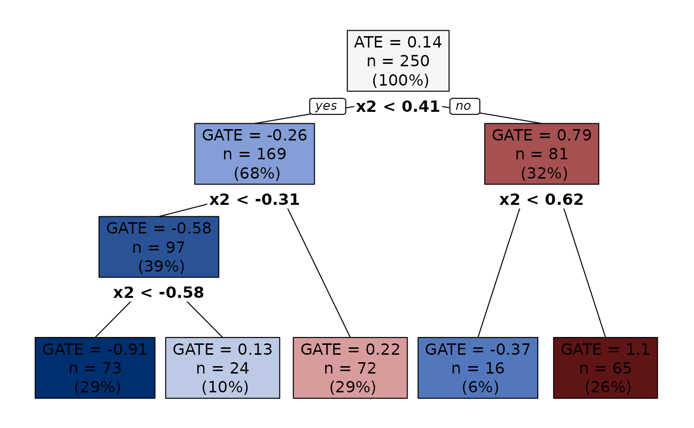

Inference

Now that we have a whole sequence of optimal groupings, we can pick the grouping associated with our preferred granularity level and call the inference_aggtree function. This function does the following:

It gets standard errors for the GATEs by estimating via OLS appropriate linear models using the honest sample. The choice of the linear model depends on the method we used when we called build_aggtree;³
It tests the null hypotheses that the differences in the GATEs across all pairs of groups equal zero. Here, we account for multiple hypotheses testing by adjusting the $p$ -values using Holm’s procedure;
It computes the average characteristics of the units in each group.

To report the results, we can print nice LATEX tables.

## Inference with 4 groups.
results <- inference_aggtree(groupings, n_groups = 4)

## LATEX.
print(results, table = "diff")
#> \begingroup
#>   \setlength{\tabcolsep}{8pt}
#>   \renewcommand{\arraystretch}{1.2}
#>   \begin{table}[b!]
#>     \centering
#>     \begin{adjustbox}{width = 1\textwidth}
#>     \begin{tabular}{@{\extracolsep{5pt}}l c c c c}
#>       \\[-1.8ex]\hline
#>       \hline \\[-1.8ex] 
#> 
#>       & \textit{Leaf 1} & \textit{Leaf 2} & \textit{Leaf 3} & \textit{Leaf 4} \\
#>       \addlinespace[2pt]
#>       \hline \\[-1.8ex] 
#> 
#>       \multirow{3}{*}{GATEs} & -0.583 & -0.366 &  0.222 &  1.117 \\
#>       & [-1.028, -0.138] & [-1.387,  0.655] & [-0.307,  0.751] & [ 0.635,  1.599] \\
#>       & \{NA, NA\} & \{NA, NA\} & \{NA, NA\} & \{NA, NA\} \\ 
#> 
#>       \addlinespace[2pt]
#>       \hline \\[-1.8ex] 
#> 
#>       \textit{Leaf 1} & NA & NA & NA & NA \\
#>             & (NA) & (NA) & (NA) & (NA) \\ 
#>       \textit{Leaf 2} & 0.22 &   NA &   NA & NA \\
#>             & (0.702) & (   NA) & (   NA) & (NA) \\ 
#>       \textit{Leaf 3} & 0.80 & 0.59 &   NA & NA \\
#>             & (0.070) & (0.635) & (   NA) & (NA) \\ 
#>       \textit{Leaf 4} & 1.70 & 1.48 & 0.90 & NA \\
#>             & (0.000) & (0.053) & (0.060) & (NA) \\ 
#> 
#>       \addlinespace[3pt]
#>       \\[-1.8ex]\hline
#>       \hline \\[-1.8ex]
#>     \end{tabular}
#>     \end{adjustbox}
#>     \caption{Point estimates and $95\%$ confidence intervals for the GATEs based on asymptotic normality (in square brackets) and on the percentiles of the bootstrap distribution (in curly braces). Leaves are sorted in increasing order of the GATEs. Additionally, the GATE differences across all pairs of leaves are displayed. $p$-values testing the null hypothesis that a single difference is zero are adjusted using Holm's procedure and reported in parenthesis under each point estimate.}
#>     \label{table_differences_gates}
#>     \end{table}
#> \endgroup

print(results, table = "avg_char")
#> \begingroup
#>   \setlength{\tabcolsep}{8pt}
#>   \renewcommand{\arraystretch}{1.1}
#>   \begin{table}[b!]
#>     \centering
#>     \begin{adjustbox}{width = 1\textwidth}
#>     \begin{tabular}{@{\extracolsep{5pt}}l c c c c c c c c }
#>       \\[-1.8ex]\hline
#>       \hline \\[-1.8ex]
#>       & \multicolumn{2}{c}{\textit{Leaf 1}} & \multicolumn{2}{c}{\textit{Leaf 2}} & \multicolumn{2}{c}{\textit{Leaf 3}} & \multicolumn{2}{c}{\textit{Leaf 4}} \\\cmidrule{2-3} \cmidrule{4-5} \cmidrule{6-7} \cmidrule{8-9} 
#>       & Mean & (S.E.) & Mean & (S.E.) & Mean & (S.E.) & Mean & (S.E.) \\
#>       \addlinespace[2pt]
#>       \hline \\[-1.8ex] 
#> 
#>       \texttt{x1} &  0.133 & (0.099) & -0.030 & (0.202) & -0.094 & (0.144) &  0.083 & (0.106) \\ 
#>       \texttt{x2} & -0.955 & (0.057) &  0.505 & (0.012) &  0.010 & (0.026) &  1.222 & (0.050) \\ 
#>       \texttt{x3} &  0.083 & (0.112) & -0.542 & (0.197) &  0.316 & (0.137) & -0.036 & (0.107) \\ 
#> 
#>       \addlinespace[3pt]
#>       \\[-1.8ex]\hline
#>       \hline \\[-1.8ex]
#>     \end{tabular}
#>     \end{adjustbox}
#>     \caption{Average characteristics of units in each leaf, obtained by regressing each covariate on a set of dummies denoting leaf membership . Standard errors are estimated via the Eicker-Huber-White estimator. Leaves are sorted in increasing order of the GATEs.}
#>     \label{table_average_characteristics_leaves}
#>     \end{table}
#> \endgroup