Short tutorial

Machine learning methods for estimating conditional average treatment effects (CATEs) produce predictions that vary across units, but this variation may reflect noise rather than genuine heterogeneity. valiCATE provides formal statistical tests to distinguish the two based on the Centered-Weighted Average Treatment Effect (CWATE) and its normalized counterpart (NCWATE).

Theory

Notation

• $Y_i$: observed outcome for unit $i$.
• $D_i$: binary treatment indicator (1 = treated, 0 = control).
• $X_i$: pre-treatment covariates.
• $\tau(X_i) := E[Y_i(1) - Y_i(0) | X_i]$: true CATE.
• $\hat{\tau}(X_i)$: ML prediction of the CATE.
• $\mu(d, x) := E[Y_i | D_i = d, X_i = x]$: conditional mean function.
• $\pi(x) := P(D_i = 1 | X_i = x)$: propensity score.
• $\Gamma_i$: AIPW pseudo-outcome, an unbiased signal for $\tau(X_i)$.
• $\omega(X_i) := \omega(\hat{\tau}(X_i))$: weight function, a centered and non-decreasing transformation of $\hat{\tau}(X_i)$.

All results assume that $\tau(X_i)$ is identified (e.g., via randomization or unconfoundedness conditional on $X_i$).

Motivating example

To see why validation matters, consider a setting where there is no treatment effect heterogeneity at all. We generate a simple randomized experiment with a single covariate and a constant (zero) treatment effect:

## Set seed and generate synthetic data.
set.seed(1986)

n <- 2000
X <- matrix(runif(n), ncol = 1, dimnames = list(NULL, "x1"))
D <- rbinom(n, size = 1, prob = 0.5)
Y <- sin(2 * pi * X[, 1]) + rnorm(n, sd = 0.5)

The true CATE is $\tau(X_i) = 0$ for every unit. Now we split the sample and fit a T-learner and a causal forest:

## Sample split.
train_idx <- sample(seq_len(n), n / 2)
val_idx <- setdiff(seq_len(n), train_idx)

## T-learner.
library(grf)

rf1 <- regression_forest(X[train_idx[D[train_idx] == 1], , drop = FALSE],
                         Y[train_idx[D[train_idx] == 1]])
rf0 <- regression_forest(X[train_idx[D[train_idx] == 0], , drop = FALSE],
                         Y[train_idx[D[train_idx] == 0]])
cates_tl <- predict(rf1, X[val_idx, , drop = FALSE])$predictions -
            predict(rf0, X[val_idx, , drop = FALSE])$predictions

## Causal forest.
cf <- causal_forest(X[train_idx, , drop = FALSE], Y[train_idx], D[train_idx])
cates_cf <- predict(cf, X[val_idx, , drop = FALSE])$predictions

Both models produce predictions that vary across units, even though the true effect is zero everywhere:

## Plot results.
library(ggplot2)

plot_df <- data.frame(
  x1 = rep(X[val_idx, 1], 2),
  cate = c(cates_tl, cates_cf),
  model = rep(c("T-learner", "Causal forest"), each = length(val_idx))
)

ggplot(plot_df, aes(x = x1, y = cate)) +
  geom_point(aes(color = "Predicted"), alpha = 0.3, size = 1) +
  geom_hline(aes(yintercept = 0, linetype = "Actual"), color = "#E63946", linewidth = 0.7) +
  scale_color_manual(name = NULL, values = c("Predicted" = "#3C78D8")) +
  scale_linetype_manual(name = NULL, values = c("Actual" = "dashed")) +
  guides(color = guide_legend(override.aes = list(alpha = 1, size = 2)),
         linetype = guide_legend(override.aes = list(color = "#E63946"))) +
  facet_wrap(~ model) +
  labs(x = expression(X[1]), y = "CATEs") +
  theme_minimal(base_size = 12) +
  theme(
    strip.text = element_text(face = "bold", size = 12),
    panel.grid.minor = element_blank(),
    legend.position = "bottom"
  )

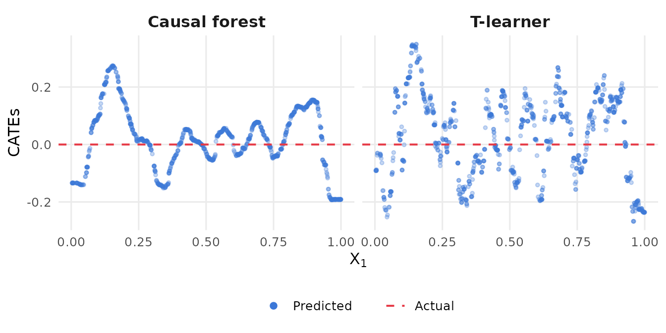
The dashed red line marks the truth ($\tau = 0$). Both models predict substantial heterogeneity that does not exist. Without a formal test, an analyst might conclude that the treatment works differently for different values of $X_1$ and proceed to target treatments accordingly. This is exactly the kind of mistake that the CWATE/NCWATE framework is designed to prevent.

The CWATE and the NCWATE

CWATE: detecting heterogeneity

Given an estimated CATE function $\hat{\tau}(\cdot)$, the natural question is whether it can be trusted: does it carry genuine information about the true CATE function $\tau(\cdot)$, or is the apparent heterogeneity an artifact of the estimation procedure? The centered weighted average treatment effect (CWATE) answers this question by summarizing the relationship between $\hat{\tau}(\cdot)$ and $\tau(\cdot)$ in a single scalar.

The CWATE is defined as $$\theta(\omega) = \text{Cov}(\omega(X_i), \tau(X_i)) = E[\omega(X_i) \tau(X_i)],$$ where the second equality follows from the centering of $\omega$. A positive CWATE indicates that units with larger $\omega(X_i)$ tend to have larger true treatment effects—the predicted heterogeneity is aligned with the true heterogeneity. A value of zero indicates no alignment.

The natural hypothesis test is one-sided: $H_0\!\!: \theta \leq 0$ against $H_1\!\!: \theta > 0$. Rejection signals that the predicted CATEs capture genuine treatment effect heterogeneity in the correct direction.

NCWATE: assessing recovery

Rejection of the one-sided CWATE null is, however, only a lower bar. A predicted CATE function may rank units correctly without coming close to the true magnitudes of treatment effects. An analyst who rejects the CWATE null still cannot conclude that $\hat{\tau}(\cdot)$ is suitable for tasks beyond ranking—such as interpreting the function through variable importance or other tools from explainable AI.

To test the stronger property that $\hat{\tau}(\cdot)$ recovers $\tau(\cdot)$, the CWATE is normalized by the value it would take if $\hat{\tau}$ were the true CATE. The resulting normalized CWATE (NCWATE) is $$\gamma(\omega) = \frac{\text{Cov}(\omega(X_i), \tau(X_i))}{\text{Cov}(\omega(X_i), \hat{\tau}(X_i))}.$$ The NCWATE equals one precisely when $\text{Cov}(\omega(X_i), \tau(X_i) - \hat{\tau}(X_i)) = 0$, that is, when the residual $\tau(X_i) - \hat{\tau}(X_i)$ is uncorrelated with $\omega(X_i)$. Pointwise recovery $\hat{\tau}(X_i) = \tau(X_i)$ is the canonical case in which this holds.

The natural hypothesis test is two-sided: $H_0\!\!: \gamma = 1$. In contrast to the CWATE test, favorable evidence consists in failure to reject: the analyst hopes that the data are consistent with $\gamma(\omega) = 1$. A non-rejection means either that $\hat{\tau}(\cdot)$ recovers $\tau(\cdot)$ pointwise, or that the residual is nonzero but uncorrelated with the chosen $\omega$. To guard against the second possibility, the analyst can interrogate $\hat{\tau}(\cdot)$ along multiple directions by varying $\omega$.

Interpretation rules

CWATE $H_0\!\!: \theta \leq 0$	NCWATE $H_0\!\!: \gamma = 1$	Interpretation
Fail to reject	(secondary)	No evidence of genuine heterogeneity.
Reject	Fail to reject	Genuine heterogeneity detected, consistent with CATE recovery.
Reject	Reject	Genuine heterogeneity detected, but the model distorts the CATEs (over- or under-prediction).

Always start with the CWATE. The NCWATE is only informative when the CWATE rejects.

Estimation and inference

The doubly-robust score

Estimation is built on the AIPW pseudo-outcome $$\Gamma_i := \mu(1, X_i) - \mu(0, X_i) + \frac{D_i}{\pi(X_i)}\big(Y_i - \mu(1, X_i)\big) - \frac{1 - D_i}{1 - \pi(X_i)}\big(Y_i - \mu(0, X_i)\big).$$ The key property is $E[\Gamma_i | X_i] = \tau(X_i)$: conditional on covariates, the score is an unbiased signal for the true CATE. In practice, $\mu$ and $\pi$ are unknown and replaced by estimates $\hat{\mu}$ and $\hat{\pi}$ obtained via $K$-fold cross-fitting, yielding the estimated score $\hat{\Gamma}_i$.

CWATE estimator

Given estimated weights $\hat{\omega}(X_i)$ and cross-fitted scores $\hat{\Gamma}_i$, the CWATE is estimated by $$\hat{\theta}_n (\hat{\omega}) = \frac{1}{n}\sum_{i=1}^n \hat{\omega}(X_i)\hat{\Gamma}_i.$$

Under regularity conditions (see Di Francesco & Knaus, 2025, Theorem 1), $$\sqrt{n}\big(\hat{\theta}_n(\hat{\omega}) - \theta(\omega)\big) \xrightarrow{d} N\big(0, V(\phi_i)\big),$$ where $\phi_i = \omega(X_i)\Gamma_i - \theta(\omega) + C_\omega(Z_i)$, with $C_\omega$ a correction term accounting for the fact that the weights are themselves estimated from the data. The variance $V(\phi_i)$ is estimated by $\hat{V}(\phi_i) = n^{-1}\sum_i \hat{\phi}_i^2$.

NCWATE estimator

The NCWATE is estimated by normalizing: $$\hat{\gamma}_n(\hat{\omega}) = \frac{\hat{\theta}_n(\hat{\omega})}{n^{-1}\sum_{i=1}^n \hat{\omega}(X_i)\hat{\tau}(X_i)}.$$

Under regularity conditions (see Di Francesco & Knaus, 2025, Theorem 2), $$\sqrt{n}\big(\hat{\gamma}_n(\hat{\omega}) - \gamma(\omega)\big) \xrightarrow{d} N\big(0, V(\psi_i)\big),$$ where $\psi_i = E[\omega(X_i)\hat{\tau}(X_i)]^{-1}\big(\omega(X_i)\big(\Gamma_i - \gamma(\omega)\hat{\tau}(X_i)\big) + C_\omega^\gamma(Z_i)\big)$, with $C_\omega^\gamma$ the corresponding correction term. The variance $V(\psi_i)$ is estimated analogously by $\hat{V}(\psi_i) = n^{-1}\sum_i \hat{\psi}_i^2$.

Training-validation split

Valid inference requires that the CATE model $\hat{\tau}$ be estimated on a training sample independent of the validation sample used to estimate $\hat{\theta}_n(\hat{\omega})$ and $\hat{\gamma}_n(\hat{\omega})$.

Weight functions

The CWATE/NCWATE framework nests several existing validation tools as special cases, each corresponding to a different weight function. Writing $F(\cdot)$ for the CDF of $\hat{\tau}(X_i)$, four natural choices are:

• BLP: $\omega(X_i) = \hat{\tau}(X_i) - E[\hat{\tau}(X_i)]$. Weights grow linearly with the prediction, so units with extreme predicted effects (high or low) drive the result. Corresponds to the slope in the Best Linear Predictor regression of Chernozhukov et al. (2018).
• AUTOC: $\omega(X_i) = -\log(1 - F(\hat{\tau}(X_i))) - 1$. A concave transformation of rank that increases slowly at the top and steeply at the bottom, so the entire ranking contributes but bottom-ranked units are upweighted. Corresponds to the Area Under the TOC Curve of Yadlowsky et al. (2021).
• QINI: $\omega(X_i) = F(\hat{\tau}(X_i)) - 1/2$. The predicted CATE rank shifted to be centered at zero. Gives roughly equal influence across the distribution, most sensitive around the median. Corresponds to the Qini coefficient of Radcliffe (2007).
• AUC-HVL: $\omega(X_i) = \log(F(\hat{\tau}(X_i)) / (1 - F(\hat{\tau}(X_i))))$. The log-odds of rank, a convex transformation that grows steeply near both tails and slowly in the middle. Emphasizes units in the extremes of the predicted CATE distribution. Corresponds to the Area Under the Cost Curve introduced in Di Francesco and Knaus (2025).

Using valiCATE

We now show how to use the package. We revisit the motivating DGP, but this time with genuine heterogeneity: $\tau(X_i) = 1 + 2 \sin(2 \pi X_{i1})$.

## Set seed and generate synthetic data.
set.seed(1986)

n <- 10000
X <- matrix(runif(n), ncol = 1, dimnames = list(NULL, "x1"))
D <- rbinom(n, size = 1, prob = 0.5)
tau <- 1 + 2 * sin(2 * pi * X[, 1])
Y <- sin(2 * pi * X[, 1]) + D * tau + rnorm(n, sd = 0.5)

CATE predictions

To illustrate the full range of possible outcomes, we compare four “estimators”: pure random noise, the oracle (the true CATEs), a T-learner, and a causal forest. We expect the noise estimator to fail both tests, the oracle to pass both, and the two ML estimators to fall somewhere in between—they should detect heterogeneity (pass CWATE) but may or may not fully recover the true CATEs (NCWATE).

As discussed in the theory section, valid inference requires that the CATE models be estimated on a training sample independent of the validation sample passed to valiCATE. We split the data 50/50 and estimate CATEs on the training half:

## Sample split.
train_idx <- sample(seq_len(n), n / 2)
val_idx <- setdiff(seq_len(n), train_idx)

## Random noise.
cates_noise <- rnorm(length(val_idx))

## Oracle (true CATEs).
cates_oracle <- tau[val_idx]

## T-learner.
rf1 <- regression_forest(X[train_idx[D[train_idx] == 1], , drop = FALSE],
                         Y[train_idx[D[train_idx] == 1]])
rf0 <- regression_forest(X[train_idx[D[train_idx] == 0], , drop = FALSE],
                         Y[train_idx[D[train_idx] == 0]])
cates_tl <- predict(rf1, X[val_idx, , drop = FALSE])$predictions -
            predict(rf0, X[val_idx, , drop = FALSE])$predictions

## Causal forest.
cf <- causal_forest(X[train_idx, , drop = FALSE], Y[train_idx], D[train_idx])
cates_cf <- predict(cf, X[val_idx, , drop = FALSE])$predictions

Running valiCATE

The main function is valiCATE(). The required inputs are the validation-sample outcomes Y, treatment indicators D, covariates X, and a named list of CATE prediction vectors cates. Each element of cates is a numeric vector of the same length as Y, and its name is used to label the model in the output. This is the only place where multiple models are passed—valiCATE handles all of them in a single call. AIPW pseudo-outcomes are estimated internally via cross-fitting, so they do not need to be supplied.

## Validate CATE predictions.
library(valiCATE)

result <- valiCATE(Y[val_idx], D[val_idx], X[val_idx, , drop = FALSE],
                   cates = list("Noise" = cates_noise,
                                "Oracle" = cates_oracle,
                                "T-learner" = cates_tl,
                                "Causal forest" = cates_cf),
                   verbose = FALSE)

Results

The results can be accessed by calling summary() on the output, which prints CWATE and NCWATE tables for all models and weight functions:

## Preview validation results.
summary(result)
#> ====================================================================== 
#> Model: Noise 
#> ====================================================================== 
#> 
#> CWATE (H0: theta <= 0, one-sided test)
#> ---------------------------------------------------------------------- 
#>   Weight       Estimate         SE           95% CI    p-value
#> ---------------------------------------------------------------------- 
#>   AUTOC         -0.0432     0.0249 [-0.0919, 0.0056]     0.9587
#>   AUC-HVL       -0.0809     0.0444 [-0.1680, 0.0061]     0.9658
#>   BLP           -0.0446     0.0249 [-0.0935, 0.0042]     0.9633
#>   QINI          -0.0125     0.0072 [-0.0266, 0.0015]     0.9596
#> 
#> NCWATE (H0: gamma = 1, two-sided test)
#> ---------------------------------------------------------------------- 
#>   Weight       Estimate         SE           95% CI    p-value
#> ---------------------------------------------------------------------- 
#>   AUTOC         -0.0474     0.0273 [-0.1010, 0.0061]     0.0000
#>   AUC-HVL       -0.0446     0.0245 [-0.0925, 0.0034]     0.0000
#>   BLP           -0.0438     0.0244 [-0.0917, 0.0041]     0.0000
#>   QINI          -0.0440     0.0252 [-0.0933, 0.0054]     0.0000
#> 
#> ====================================================================== 
#> Model: Oracle 
#> ====================================================================== 
#> 
#> CWATE (H0: theta <= 0, one-sided test)
#> ---------------------------------------------------------------------- 
#>   Weight       Estimate         SE           95% CI    p-value
#> ---------------------------------------------------------------------- 
#>   AUTOC          1.1717     0.0167 [1.1390, 1.2044]     0.0000
#>   AUC-HVL        2.3514     0.0291 [2.2944, 2.4083]     0.0000
#>   BLP            1.9787     0.0295 [1.9210, 2.0364]     0.0000
#>   QINI           0.4031     0.0048 [0.3936, 0.4125]     0.0000
#> 
#> NCWATE (H0: gamma = 1, two-sided test)
#> ---------------------------------------------------------------------- 
#>   Weight       Estimate         SE           95% CI    p-value
#> ---------------------------------------------------------------------- 
#>   AUTOC          0.9992     0.0133 [0.9733, 1.0252]     0.9536
#>   AUC-HVL        1.0020     0.0118 [0.9788, 1.0252]     0.8669
#>   BLP            0.9980     0.0109 [0.9766, 1.0195]     0.8559
#>   QINI           0.9984     0.0111 [0.9767, 1.0201]     0.8847
#> 
#> ====================================================================== 
#> Model: T-learner 
#> ====================================================================== 
#> 
#> CWATE (H0: theta <= 0, one-sided test)
#> ---------------------------------------------------------------------- 
#>   Weight       Estimate         SE           95% CI    p-value
#> ---------------------------------------------------------------------- 
#>   AUTOC          1.1487     0.0170 [1.1154, 1.1820]     0.0000
#>   AUC-HVL        2.3191     0.0293 [2.2616, 2.3766]     0.0000
#>   BLP            1.9962     0.0299 [1.9377, 2.0548]     0.0000
#>   QINI           0.4003     0.0048 [0.3909, 0.4097]     0.0000
#> 
#> NCWATE (H0: gamma = 1, two-sided test)
#> ---------------------------------------------------------------------- 
#>   Weight       Estimate         SE           95% CI    p-value
#> ---------------------------------------------------------------------- 
#>   AUTOC          0.9516     0.0132 [0.9258, 0.9774]     0.0002
#>   AUC-HVL        0.9667     0.0118 [0.9435, 0.9899]     0.0049
#>   BLP            0.9779     0.0109 [0.9565, 0.9992]     0.0422
#>   QINI           0.9762     0.0110 [0.9546, 0.9977]     0.0299
#> 
#> ====================================================================== 
#> Model: Causal forest 
#> ====================================================================== 
#> 
#> CWATE (H0: theta <= 0, one-sided test)
#> ---------------------------------------------------------------------- 
#>   Weight       Estimate         SE           95% CI    p-value
#> ---------------------------------------------------------------------- 
#>   AUTOC          1.1514     0.0167 [1.1186, 1.1841]     0.0000
#>   AUC-HVL        2.3261     0.0289 [2.2695, 2.3827]     0.0000
#>   BLP            1.9934     0.0297 [1.9352, 2.0517]     0.0000
#>   QINI           0.4011     0.0048 [0.3917, 0.4105]     0.0000
#> 
#> NCWATE (H0: gamma = 1, two-sided test)
#> ---------------------------------------------------------------------- 
#>   Weight       Estimate         SE           95% CI    p-value
#> ---------------------------------------------------------------------- 
#>   AUTOC          0.9606     0.0130 [0.9351, 0.9862]     0.0025
#>   AUC-HVL        0.9763     0.0117 [0.9534, 0.9992]     0.0429
#>   BLP            0.9835     0.0109 [0.9621, 1.0048]     0.1294
#>   QINI           0.9825     0.0110 [0.9610, 1.0040]     0.1102

CWATE (step 1—is there genuine heterogeneity?).

• Noise: all CWATE $p$-values are large, so $H_0\!\!: \theta \leq 0$ is not rejected. Random predictions carry no information about the true treatment effects, and the test correctly detects this.
• Oracle: all CWATE $p$-values are small, so $H_0\!\!: \theta \leq 0$ is rejected. The true CATEs are, by construction, perfectly aligned with the true heterogeneity, and the test correctly supports this.
• T-learner and causal forest: both also reject across all weight functions, indicating that their predicted heterogeneity is genuine.

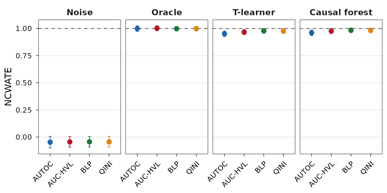
NCWATE (step 2—does the model recover the true CATEs?).

• Noise: The NCWATE is only meaningful for estimators that pass the CWATE test, so we skip the noise estimator.
• Oracle: NCWATE estimates are close to 1 with large $p$-values, so $H_0\!\!: \gamma = 1$ is not rejected. This is the expected benchmark: the true CATEs trivially recover themselves.
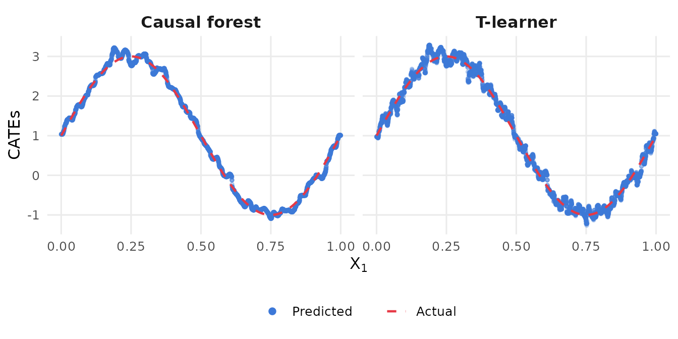
• T-learner and causal forest: NCWATE estimates are close to 1 for both models, but the causal forest is slightly more consistent: $H_0\!\!: \gamma = 1$ is rejected for two weight functions with the T-learner, while only one rejection occurs for the causal forest. Overall, both models are largely consistent with recovering the true CATEs in this simple DGP, with a slight edge for the causal forest.

Since we are using synthetic data, we can actually visualize the recovery by comparing predicted CATEs against the truth:

## Plot true and predicted CATEs.
plot_df <- data.frame(
  x1 = rep(X[val_idx, 1], 2),
  cate = c(cates_tl, cates_cf),
  model = rep(c("T-learner", "Causal forest"), each = length(val_idx))
)

ggplot(plot_df, aes(x = x1, y = cate)) +
  geom_point(aes(color = "Predicted"), alpha = 0.3, size = 1) +
  geom_line(aes(y = rep(tau[val_idx], 2), linetype = "Actual"), color = "#E63946",
            linewidth = 0.8) +
  scale_color_manual(name = NULL, values = c("Predicted" = "#3C78D8")) +
  scale_linetype_manual(name = NULL, values = c("Actual" = "dashed")) +
  guides(color = guide_legend(override.aes = list(alpha = 1, size = 2)),
         linetype = guide_legend(override.aes = list(color = "#E63946"))) +
  facet_wrap(~ model) +
  labs(x = expression(X[1]), y = "CATEs") +
  theme_minimal(base_size = 12) +
  theme(
    strip.text = element_text(face = "bold", size = 12),
    panel.grid.minor = element_blank(),
    legend.position = "bottom"
  )

The summary method can also produce a ready-to-compile LaTeX table by setting latex = TRUE. Compilation requires the LaTeX packages booktabs, float, and adjustbox.

## Print LATEX table.
summary(result, latex = TRUE)

Alternatively, the plot method produces a coefficient plot with point estimates and confidence intervals for each weight function, faceted by model. We first plot the CWATE estimates:

## Coefficient plot of CWATE estimates.
plot(result)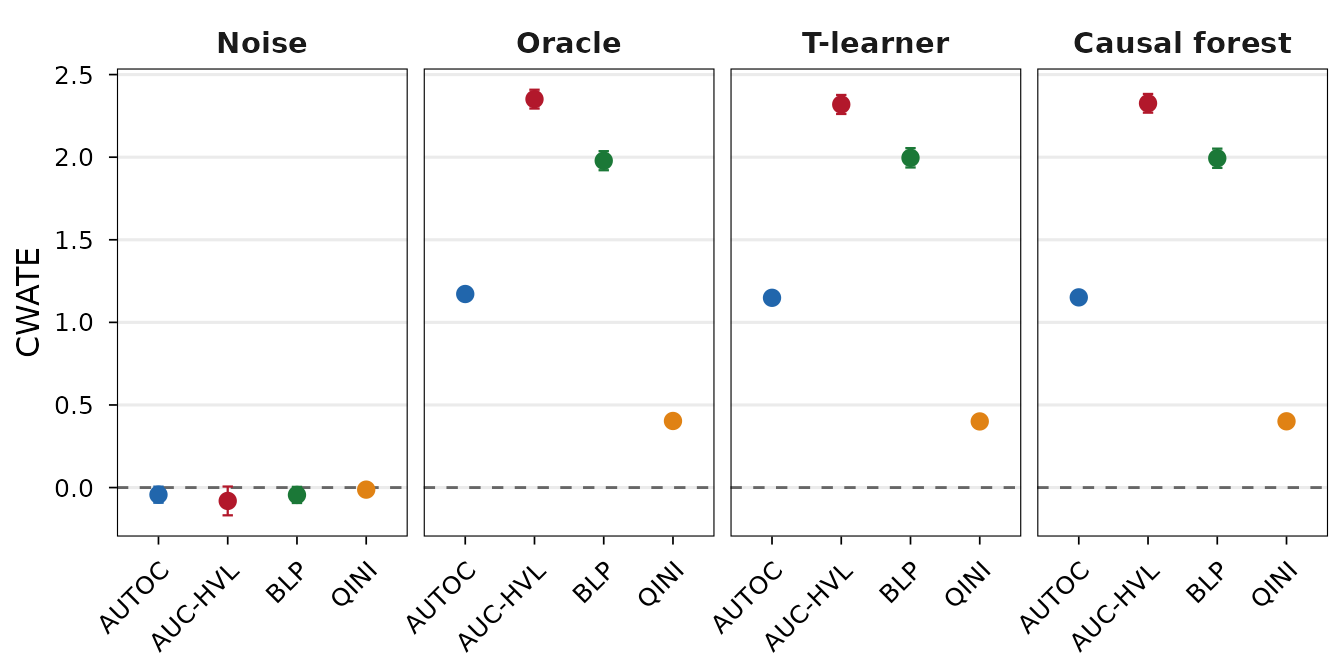

And then the NCWATE estimates:

## Coefficient plot of NCWATE estimates.
plot(result, type = "ncwate")