Short Tutorial

In this tutorial, we show how to use the valiCATE package to validate machine learning models for the conditional average treatment effects (CATEs).

Before diving in the technical details, we need to define notation:

• $Y_i$ → Observed outcome;
• $D_i \in \{ 0, 1\}$ → Treatment indicator;
• $X_i$ → Covariate vector;
• $\mu ( X_i ) := \mathbb{E} [ Y_i | X_i ]$ → Conditional mean of $Y_i$ given $X_i$;
• $\mu (d, X_i ) := \mathbb{E} [ Y_i | X_i, D_i = d ]$ → Conditional mean of $Y_i$ given $X_i$ for subgroup $D_i = d$;
• $p ( X_i ) := \mathbb{P} [ D_i = 1 | X_i ]$ → Propensity score;
• $w ( X_i ) := \frac{1}{p ( X_i ) [ 1 - p ( X_i )]}$ → Propensity score weights;
• $H_i := w ( X_i ) [ D_i - p (X_i) ]$ → Horvitz-Thompson operator;
• $\Gamma_i := \mu_1 ( X_i ) - \mu_0 ( X_i ) + \frac{D_i [ Y_i - \mu_1 ( X_i ) ]}{p ( X_i )} - \frac{[ 1 - D_i ] [ Y_i - \mu_0 ( X_i ) ]}{1 - p ( X_i )}$ → Doubly-robust (or AIPW) score;
• $\tau := \mathbb{E} [ Y_i ( 1 ) - Y_i ( 0 ) ]$ → Average treatment effect (ATE);
• $\tau ( X_i ) := \mathbb{E} [ Y_i ( 1 ) - Y_i ( 0 ) | X_i ]$ → CATE.

Throughout the rest of the tutorial, we assume SUTVA and a randomized treatment assignment.

Motivating Example

We illustrate the usage of the valiCATE package with simulated data:

• $X_{i} \sim \mathcal{U} ( 0, 1 )$ single uniformly distributed covariate;

• $D_i \sim Bernoulli(0.4)$ randomly assigned treatment;

• $Y_i = X_i + 0 \times D_i + \varepsilon_i$ with $\varepsilon_i \sim \mathcal{N} ( 0, 5 )$;

This implies a homogeneous zero effect, i.e. $\tau ( X_i ) = 0$.

## Generate data.
set.seed(1986)

n <- 500
k <- 1

X <- matrix(runif(n * k), ncol = k)
colnames(X) <- paste0("x", seq_len(k))
D <- rbinom(n, size = 1, prob = 0.4)
mu0 <- X[, 1]
mu1 <- X[, 1]
Y <- mu0 + D * (mu1 - mu0) + rnorm(n, sd = sqrt(5))

To achieve valid inference, we randomly partition our data set into two subsamples:

1. a training sample for estimating the CATEs, and

2. a validation sample to validate the estimated heterogeneity.

We explore two distinct models for CATE estimation: a T-learner employing honest regression forests as base learners, and an honest causal forest.

## Sample split.
train_idx <- sample(c(TRUE, FALSE), length(Y), replace = TRUE)

X_tr <- matrix(X[train_idx, ])
X_val <- matrix(X[!train_idx, ])

D_tr <- D[train_idx]
D_val <- D[!train_idx]

Y_tr <- Y[train_idx]
Y_val <- Y[!train_idx]

## CATEs estimation.
# T-learner.
forest_treated <- regression_forest(as.matrix(X_tr[D_tr == 1, ]), Y_tr[D_tr == 1])
forest_control <- regression_forest(as.matrix(X_tr[D_tr == 0, ]), Y_tr[D_tr == 0])
cates_val_t <- predict(forest_treated, X_val)$predictions - predict(forest_control, X_val)$predictions 

# Causal forest.
forest <- causal_forest(X_tr, Y_tr, D_tr) 
cates_val_cf <- predict(forest, X_val)$predictions 

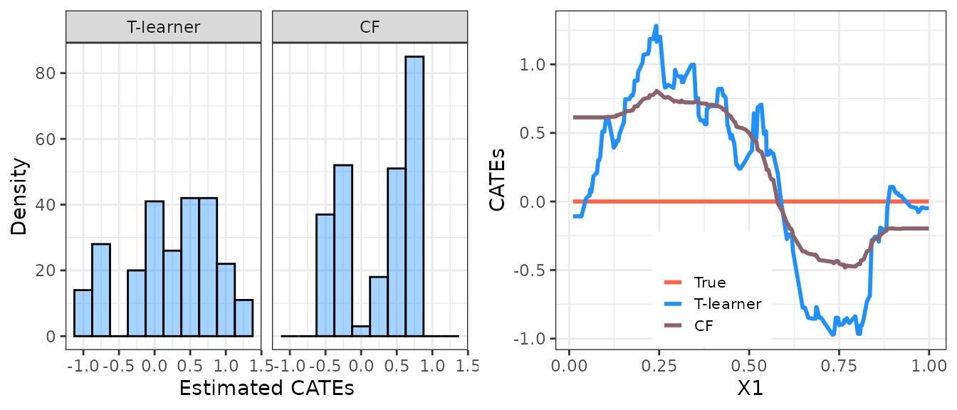
Let’s display the distribution of the out-of-sample CATE predictions. Observing the histograms below, one might infer the presence of heterogeneity in the treatment effects. However, substantial variation in predictions does not definitively indicate heterogeneous effects, as this variation may be attributed to estimation noise messing with our results (precisely what is occurring in our example!).

These complexities arise because the application of machine learning tools to estimate heterogeneous treatment effects may produce low-quality CATE estimates (see, e.g., the figure below, where we compare true and estimated CATEs). It is therefore crucial to employ appropriate procedures to validate the estimated CATE models and assess whether systematic heterogeneity is detected. This is the purpose of the valiCATE package.

## Out-of-sample predicted CATEs.
p1 <- data.frame("cates" = cates_val_t, "estimator" = "T-learner") %>%
  bind_rows(data.frame("cates" = cates_val_cf, "estimator" = "CF")) %>%
  ggplot(aes(x = cates)) +
  geom_histogram(color = "black", fill = "dodgerblue", alpha = 0.4, bins = 10) + 
  facet_grid(cols = vars(factor(estimator, levels = c("T-learner", "CF")))) +
  xlab("Estimated CATEs") + ylab("Density") +
  theme_bw() + 
  theme(plot.title = element_text(hjust = 0.5), legend.position = "none")

## True and estimated CATEs.
p2 <- data.frame("x1" = X_val, "true_cates" = mu1[!train_idx] - mu0[!train_idx], "cates_t" = cates_val_t, "cates_cf" = cates_val_cf) %>%
  melt(id.vars = "x1") %>%
  ggplot(aes(x = x1, y = value, group = variable, color = variable)) + 
  geom_line(linewidth = 1) +
  scale_color_manual(name = "", labels = c("True", "T-learner", "CF"), values = c("tomato", "dodgerblue", "pink4")) +
  xlab("X1") + ylab("CATEs") +  
  theme_bw() + 
  theme(plot.title = element_text(hjust = 0.5), legend.position = c(0.40, 0.18), legend.text = element_text(size = 8), legend.key.size = unit(0.4, 'cm'))
#> Warning: A numeric `legend.position` argument in `theme()` was deprecated in ggplot2
#> 3.5.0.
#> ℹ Please use the `legend.position.inside` argument of `theme()` instead.
#> This warning is displayed once every 8 hours.
#> Call `lifecycle::last_lifecycle_warnings()` to see where this warning was
#> generated.

## Grid.
grid.arrange(p1, p2, ncol = 2)

Validation

The validation of the estimated CATE models focuses on three key targets:

• Best Linear Predictor (BLP) of the actual CATEs using the estimated CATEs;
• Sorted Group Average Treatment Effects (GATES);
• Rank-Weighted Average Treatment Effects (RATEs) induced by the estimated CATEs.

This section offers an overview of these targets. The discussion is loosely based on Chernozhukov et al. (2017), Yadlowsky et al. (2021), and Imai and Li (2022).¹

Keep in mind that achieving valid inference necessitates a training-validation sample split, akin to that performed in the Motivating Example. Then, for any fixed $\hat{\tau} ( \cdot )$ obtained using only the training sample, our targets of interest are estimated using observations solely from the validation sample.

Best Linear Predictor

The BLP of the actual CATEs using the estimated CATEs is defined as follows:

$$BLP [\tau ( X_i ) | \hat{\tau} ( X_i )] := \beta_1 + \beta_2 [ \hat{\tau} ( X_i ) - \mathbb{E} [ \hat{\tau} ( X_i ) ] ]$$

with $\beta_1 = \mathbb{E} [ \tau ( X_i ) ]$ and $\beta_2 = Cov [ \tau ( X_i ), \hat{\tau} ( X_i ) ] / Var [ \hat{\tau} ( X_i ) ] = \mathbb{E} \left[ \frac{\hat{\tau} ( X_i ) - \mathbb{E} [\hat{\tau} ( X_i ) ]}{Var [ \hat{\tau} ( X_i ) ]} \tau ( X_i ) \right]$.

Our primary focus is on $\beta_2$. Notice that $\beta_2 = 0$ if either a) the effects are homogeneous or b) our CATE estimates are unreliable. Therefore, rejecting the hypothesis $\beta_2 = 0$ would suggest both heterogeneous effects and reliable CATE estimates.² As a byproduct, $\beta_1$ identifies the ATE.

The valiCATE package estimates the BLP using three distinct strategies, each entailing the fitting of an appropriate regression model.^{3 4}

• Weighted Residuals:

$$Y_i = \beta_1 [ D_i - p ( X_i ) ] + \beta_2 \{ [ D_i - p ( X_i ) ] [ \hat{\tau} ( X_i ) - \mathbb{E}_n [ \hat{\tau} ( X_i ) ] ] \} + \epsilon_i$$ with the model fitted via WLS using weights $w ( X_i)$ and $\mathbb{E}_n$ denoting the sample average operator.

• Horvitz-Thompson

$$H_i Y_i = \beta_1 + \beta_2 \{ \hat{\tau} ( X_i ) - \mathbb{E}_{n, V} [ \hat{\tau} ( X_i ) ] \} + \epsilon_i$$ with the model fitted via OLS.

• AIPW

$$\hat{\Gamma}_i = \beta_1 + \beta_2 \{ \hat{\tau} ( X_i ) - \mathbb{E}_{n, V} [ \hat{\tau} ( X_i ) ] \} + \epsilon_i$$ with the model fitted via OLS and the doubly-robust scores $\Gamma_i$ constructed either via cross-fitting in the validation sample or using the out-of-sample predictions of the nuisance models trained in the training sample.

Sorted Group Average Treatment Effects

The GATES are defined as follows:

$$\gamma_k := \mathbb{E} [ \tau ( X_i ) | \hat{\ell}_{k - 1} \leq \hat{\tau} ( X_i ) < \hat{\ell}_k ], \,\,\, k = 1, \dots, K$$

with the groups formed by cutting the distribution of $\hat{\tau} ( \cdot )$ into $K$ bins using the empirical quantiles of $\hat{\tau} ( \cdot )$$\{ \hat{\ell}_k \}_{k = 1}^K$.

Our main objective is to test specific hypotheses regarding the GATES, enabling us to determine whether we detect systematic heterogeneity or merely estimation noise. For example, we can examine whether all GATES are equal ($\gamma_1 = \gamma_2 = \dots = \gamma_K$) or if the difference between the largest and smallest GATES is zero ($\gamma_K = \gamma_1$).⁵ As a byproduct, the GATES quantify the degree to which effects vary across groups, thus offering an immediate visualization of the estimated heterogeneity *although disparities in the point estimates can emerge merely due to estimation noise).

The valiCATE package estimates the GATES using four different strategies, three of which involve fitting an appropriate regression model, while the fourth relies on a nonparametric approach.^{6 7}

Weighted Residuals

$$Y_i = \sum_{k = 1}^K \gamma_k [ D_i - p ( X_i ) ] \mathbb{1} ( \hat{\ell}_{k - 1} \leq \hat{\tau} ( X_i ) < \hat{\ell}_k ) + \epsilon_i$$

with the model fitted via WLS using weights $w ( X_i)$.

Horvitz-Thompson

$$H_i Y_i = \sum_{k = 1}^K \gamma_k \mathbb{1} ( \hat{\ell}_{k - 1} \leq \hat{\tau} ( X_i ) < \hat{\ell}_k ) + \epsilon_i$$

with the model fitted via OLS.

AIPW

$$\hat{\Gamma}_i = \sum_{k = 1}^K \gamma_k \mathbb{1} ( \hat{\ell}_{k - 1} \leq \hat{\tau} ( X_i ) < \hat{\ell}_k ) + \epsilon_i$$

with the model fitted via OLS and the doubly-robust scores $\Gamma_i$ constructed either via cross-fitting in the validation sample or using the out-of-sample predictions of the nuisance models trained in the training sample.

Nonparametric

$$\hat{\gamma}_k = \frac{K}{\sum_{i = 1}^n D_i} \sum_{i = 1}^n Y_i D_i \mathbb{1} ( \hat{\ell}_{k - 1} \leq \hat{\tau} ( X_i ) < \hat{\ell}_k ) - \frac{K}{\sum_{i = 1}^n [ 1 - D_i ]} \sum_{i = 1}^n Y_i [ 1 - D_i ] \mathbb{1} ( \hat{\ell}_{k - 1} \leq \hat{\tau} ( X_i ) < \hat{\ell}_k )$$

Rank-Weighted Average Treatment Effects

The RATE induced by the estimated CATEs is defined as follows:

$$\theta_{\alpha} ( \hat{\tau} ) := \int_0^1 \alpha ( u ) TOC ( u; \hat{\tau} ) d u$$ where:

$$TOC (u; \hat{\tau}) := \mathbb{E} [ Y_i ( 1 ) - Y_i ( 0 ) \mid F ( \hat{\tau} ( X_i )) \geq 1 - u ] - \mathbb{E} [ Y_i ( 1 ) - Y_i ( 0 ) ]$$ with $F ( \cdot )$ the cumulative distribution function of $\hat{\tau} ( \cdot )$, $0 < u \leq 1$, and $\alpha : ( 0, 1 ] \rightarrow \mathcal{R}$ a generic weight function.

The RATE offers a measure of how effectively our estimated CATEs prioritize units for treatment in terms of intervention benefit. The concept involves considering $\hat{\tau} ( \cdot )$ as a “prioritization rule” that arranges units $i = 1, ..., n$ in order $j = 1, ..., n$ based on their estimated CATEs, such as by giving priority to units with the largest estimated CATEs.^{8 9}

Our primary focus is to test the hypothesis $\theta_{\alpha} ( \hat{\tau} ) = 0$, which holds true if either a) the effects are homogeneous or b) our CATE estimates are unreliable. Thus, rejecting the hypothesis $\theta_{\alpha} ( \hat{\tau} ) = 0$ would indicate both heterogeneous effects and reliable CATE estimates.¹⁰

The valiCATE package estimates the TOCs and the RATE using the following sample-averaging estimators:

$$\widehat{TOC} ( u; \hat{\tau} ) = \frac{1}{ \lfloor u n \rfloor } \sum_{j = 1}^{\lfloor u n \rfloor} \hat{\Gamma}_{i ( j )} - \frac{1}{n} \sum_{i = 1}^n \hat{\Gamma}_i$$$$\hat{\theta}_{\alpha} ( \hat{\tau} ) = \frac{1}{n} \sum_{j = 1}^n \alpha \left( \frac{j}{n} \right) \widehat{TOC} \left( \frac{j}{n}; \hat{\tau} \right)$$ where we let $i ( j )$ be the mapping from rank $j$ to unit $i$ (e.g., $i ( 1 )$ returns the most-prioritized unit, and $i ( n )$ returns the least-prioritized unit) and the doubly-robust scores $\Gamma_i$ are constructed either via cross-fitting in the validation sample or using the out-of-sample predictions of the nuisance models trained in the training sample.

The valiCATE package considers two distinct weighting functions, each corresponding to a different RATE:

• $\alpha ( u ) = 1$ → Area under the TOC curve (AUTOC)
• $\alpha ( u ) = u$ → Qini coefficient (QINI)

The half-sample bootstrap procedure is employed to estimate the standard error of $\hat{\theta}_{\alpha} ( \cdot )$.

Code

Calling the Main Function

To estimate the BLP, GATES, and RATEs, we use the valiCATE function. When calling this function, we must provide our sample using the first six arguments: Y_tr and Y_val for the observed outcomes, D_tr and D_val for the treatment assignment, and X_tr and X_val for the covariates of units in the training and validation subsamples. Furthermore, it is necessary to supply our CATE predictions on the validation sample using the cates_val argument. This argument should consist of a named list, with each element storing a vector of CATE predictions produced by a specific model. We can choose our preferred names for the elements, keeping in mind that these names will be used to display and plot the results. We have already defined most of the arguments mentioned in this paragraph in our Motivating Example above. Below, we construct the cates_val list that stores the out-of-sample predictions produced by the T-learner and the causal forest.

The valiCATE function can implement all the BLP and GATES estimation strategies outlined in the Validation section. Users can choose their preferred strategies by controlling the strategies argument. However, this choice has no impact on RATEs estimation, which are always estimated using the sample-averaging estimators discussed above. Furthermore, the nonparametric strategy for GATES estimation is always implemented. Below, we opt to implement only the weighted residuals and the horvitz-thompson strategies.

Users can choose to include the additional constructed covariates discussed in footnotes 4 and 7 by controlling the denoising argument. However, this choice does not impact RATEs estimation or the results from the nonparametric GATES estimation strategy. Below, we decide not to include any constructed covariate.

Specific nuisance functions are necessary to conduct the analysis outlined in the Validation section. Users can provide predictions on the validation sample of $p ( \cdot )$, $\mu ( \cdot )$, $\mu_0 ( \cdot )$, and $\mu_1 ( \cdot )$ using the optional arguments pscore_val, mu_val, mu0_val, and mu1_val, respectively. It is important to note that these predictions must be generated by models estimated using only the training sample. If not supplied by the user, these functions are internally estimated via honest regression forests using only the training sample. In our Motivating Example, we know the actual propensity score, which is constant at $0.4$ for all units.¹¹ We provide these values in the call below and allow the function to internally estimate the other nuisances.

Finally, we have five additional optional arguments. n_groups controls the number of groups formed for the GATES analysis. beneficial specifies how to rank units for the RATE estimation (according to either increasing or decreasing values of the estimated CATEs). n_boot determines the number of bootstrap replications used to estimate the standard error of the estimated RATEs. crossfit_dr controls whether the doubly-robust scores are constructed via cross-fitting in the validation sample or using the out-of-sample predictions of the nuisance models trained in the training sample. verbose controls whether the valiCATE function should print progress status on the console. Below, we use the default settings of 5 groups, where the treatment is considered beneficial, 200 bootstrap replications, and cross-fitting in the validation sample. We prevent the function from printing progress updates.

## Define arguments.
cates_val <- list("T-learner" = cates_val_t,
                  "CF" = cates_val_cf)

strategies <- c("WR", "HT")
denoising <- "none"

pscore_val <- rep(0.4, length(Y_val)) # True propensity scores.

## Call main function.
validation <- valiCATE(Y_tr, Y_val, D_tr, D_val, X_tr, X_val, cates_val, strategies = strategies, denoising = denoising, pscore_val = pscore_val, verbose = FALSE)

Results

The summary method enables us to visualize the results of the BLP estimation when we set the target argument to BLP. The latex argument determines whether the raw results or LATEX code for a table will be displayed in the console. Additionally, we can use the which_models argument to select which results to display, which is useful to avoid a lengthy output. Since we have estimated a small number of models, we opt for the default option and display all results.

We consistently fail to reject the hypothesis $\beta_2 = 0$, suggesting that either the effects are homogeneous or our CATE estimates are unreliable (both are true in our Motivating Example). Given our knowledge of the DGP, the results indicate that both models produce unreliable estimates. Overall, the BLP analysis suggests that the heterogeneity implied by the distribution of the estimated CATEs might be merely estimation noise.

## BLP summary.
summary(validation, target = "BLP") # Try 'latex = TRUE'.
#> 
#> ── BLP RESULTS ─────────────────────────────────────────────────────────────────
#> 
#> ── T-learner ──
#> 
#>       MODEL       |       ATE       |       HET       
#> ----------------- | --------------- | --------------- | 
#>      wr_none      |       0.45      |      -0.37      | 
#>                   | [-0.117, 1.009] | [-1.325, 0.583] | 
#>      ht_none      |       0.47      |      -0.41      | 
#>                   | [-0.118, 1.057] | [-1.398, 0.581] |
#> ── CF ──
#>       MODEL       |       ATE       |       HET       
#> ----------------- | --------------- | --------------- | 
#>      wr_none      |       0.44      |      -0.66      | 
#>                   | [-0.121, 1.006] | [-1.888, 0.563] | 
#>      ht_none      |       0.47      |      -0.73      | 
#>                   | [-0.118, 1.056] | [-2.017, 0.562] |
#> ────────────────────────────────────────────────────────────────────────────────

We can call the summary method with the target argument set to GATES to visualize the results of the GATES hypotheses testing, with the other arguments functioning as before. To visualize GATES point estimates and confidence intervals, we can call the plot method and set the target argument to GATES. Similarly to the summary method, we could utilize the which_models argument to select which results to display, although it is not necessary in this context.

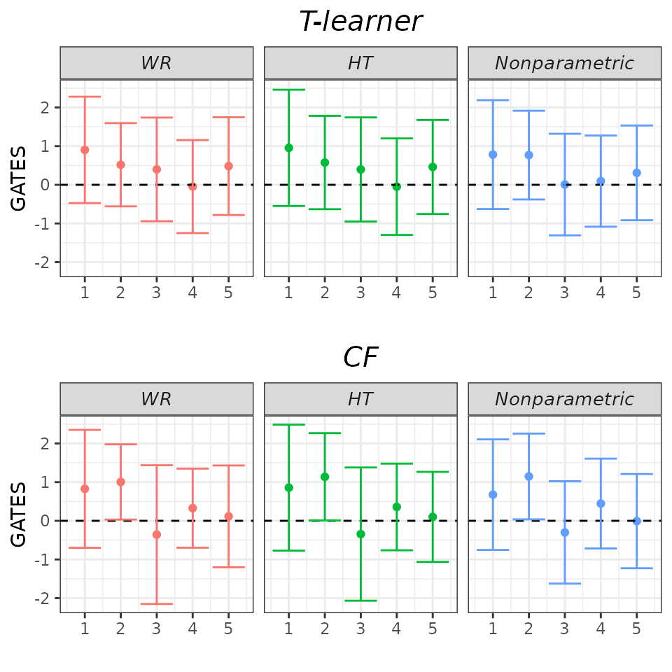
Almost all GATES confidence intervals encompass zero, indicating that no group is affected by the treatment (true in our Motivating Example!). The estimated $p$-values for testing the hypotheses that all GATES are equal and that the most and least affected groups exhibit the same response to treatment are large, resulting in a failure to reject these hypotheses. This GATES analysis offers additional evidence that the effects are not heterogeneous.

## GATES summary.
summary(validation, target = "GATES") # Try 'latex = TRUE'.
#> 
#> ── HYPOTHESIS TESTING RESULTS (p-values) ───────────────────────────────────────
#> 
#> ── T-learner ──
#> 
#>       MODEL       |       GATES_1 = GATES_2 = ... = GATES_K       |       GATES_K = GATES_1       
#> ----------------- | --------------------------------------------- | ----------------------------- | 
#>      wr_none      |                     0.895                     |             0.659             | 
#>      ht_none      |                     0.895                     |             0.617             | 
#>      imai_li      |                     0.935                     |               NA              |
#> ── CF ──
#>       MODEL       |       GATES_1 = GATES_2 = ... = GATES_K       |       GATES_K = GATES_1       
#> ----------------- | --------------------------------------------- | ----------------------------- | 
#>      wr_none      |                     0.640                     |             0.489             | 
#>      ht_none      |                     0.586                     |             0.460             | 
#>      imai_li      |                     0.641                     |               NA              |
#> ────────────────────────────────────────────────────────────────────────────────

plot(validation, target = "GATES")

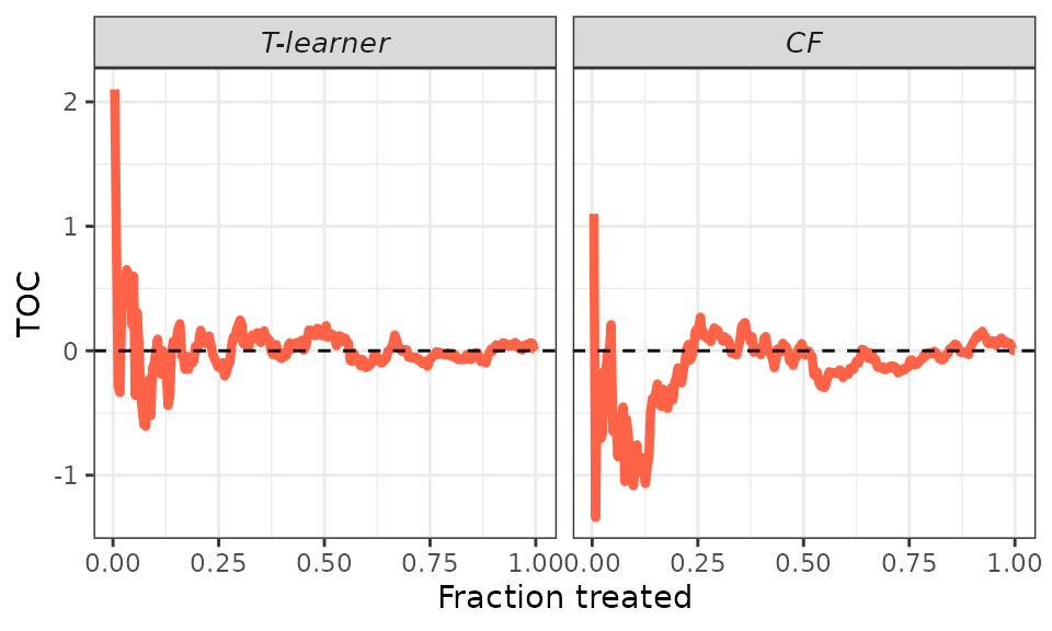
Lastly, calling the summary method with the target argument set to RATE enables us to visualize the results of the RATE estimation. To plot the estimated TOC curve, we can call the plot method and set the target argument to TOC. The AUTOC coefficient corresponds to the area under the TOC curve, while the QINI coefficient corresponds to the area under the curve $u \times TOC (u; \hat{\tau})$.

Overall, the results align with those of the BLP analysis. We consistently fail to reject the hypothesis $\theta_{\alpha} ( \hat{\tau} ) = 0$, suggesting that either the effects are homogeneous or our CATE estimates are unreliable. Given our knowledge of the DGP, the results indicate that both models produce unreliable estimates.

## RATEs summary.
summary(validation, target = "RATE") # Try 'latex = TRUE'.
#> 
#> ── RATEs RESULTS ───────────────────────────────────────────────────────────────
#> 
#> ── T-learner ──
#> 
#>       WEIGHT       |       RATE       | 
#> ------------------ | ---------------- |  
#>        autoc       |       0.02       | 
#>                    |  [-0.455, Infty] | 
#>        qini        |       0.00       | 
#>                    |  [-0.150, Infty] |
#> ── CF ──
#>       WEIGHT       |       RATE       | 
#> ------------------ | ---------------- |  
#>        autoc       |       -0.12      | 
#>                    |  [-0.544, Infty] | 
#>        qini        |       -0.02      | 
#>                    |  [-0.157, Infty] |

plot(validation, target = "TOC")

---

1. Complete references to these papers are listed in the home page.↩︎

2. Failing to reject this hypothesis suggests either there is no heterogeneity or our CATE estimates are not reliable. Without further evidence, we cannot disentangle this ambiguity. Check the hypotheses testing vignette for more details.↩︎

3. The linear regressions are used for estimation purposes. The identification hinges on linear projections defined at the population level, with the linear regressions constituting their sample analogs.↩︎

4. For each of these alternatives, additional constructed covariates not necessary for identifying the targets can be included in the regressions to reduce estimation variance. Details can be found in the denoising vignette.↩︎

5. Check the hypotheses testing vignette for details.↩︎

6. See footnote 3.↩︎

7. For each of the parametric alternatives, additional constructed covariates not necessary for identifying the targets can be included in the regressions to reduce estimation variance. Details can be found in the denoising vignette.↩︎

8. If the treatment is harmful, we prioritize units with the lowest estimated CATEs.↩︎

9. Prioritization rules can be derived from alternatives approaches, such as risk-based rules. However, our focus here is on CATE-based rules, as we intend to utilize the RATEs to valdiate our estimated CATE models.↩︎

10. See footnote 2.↩︎

11. It is important to note that most methodologies implemented here are valid only under randomized experiments, where $p ( \cdot )$ is known. The only exception is the AIPW strategy, which is valid under unconfoundedness.↩︎