Causal Inference for Qualitative Outcomes under Difference-in-Differences

Fit two-group/two-period models for qualitative outcomes to estimate the probabilities of shift on the treated.

causalQual_did(Y_pre, Y_post, D)

Arguments

Y_pre: Qualitative outcome before treatment. Must be labeled as $\{1, 2, \dots\}$.
Y_post: Qualitative outcome after treatment. Must be labeled as $\{1, 2, \dots\}$.
D: Binary treatment indicator.

Value

An object of class causalQual.

Details

Under a difference-in-difference design, identification requires that the probabilities time shift for $Y_{is} (0)$ for class $m$ evolve similarly for the treated and control groups (parallel trends on the probability mass functions of $Y_{is}(0)$). If this assumption holds, we can recover the probability of shift on the treated for class $m$:

$$\delta_{m, T} := P(Y_{it} (1) = m | D_i = 1) - P(Y_{it}(0) = m | D_i = 1).$$

causalQual_did applies, for each class $m$, the canonical two-group/two-period method to the binary variable $1(Y_{is} = m)$. Specifically, consider the following linear model:

$$1(Y_{is} = m) = D_i \beta_{m1} + 1(s = t) \beta_{m2} + D_i 1(s = t) \beta_{m3} + \epsilon_{mis}.$$

The OLS estimate $\hat{\beta}_{m3}$ of $\beta_{m3}$ is our estimate of the probability shift on the treated for class m. Standard errors are clustered at the unit level and used to construct conventional confidence intervals.

References

Di Francesco, R., and Mellace, G. (2025). Causal Inference for Qualitative Outcomes. arXiv preprint arXiv:2502.11691. doi:10.48550/arXiv.2502.11691 .

Author

Riccardo Di Francesco

Examples

## Generate synthetic data.
set.seed(1986)

data <- generate_qualitative_data_did(100, assignment = "observational",
                                      outcome_type = "ordered")

Y_pre <- data$Y_pre
Y_post <- data$Y_post
D <- data$D

## Estimate probabilities of shift on the treated.
fit <- causalQual_did(Y_pre, Y_post, D)

summary(fit)
#> 
#> ── CAUSAL INFERENCE FOR QUALITATIVE OUTCOMES ───────────────────────────────────
#> 
#> ── Research design ──
#> 
#> Identification:          Difference-in-Differences 
#> Estimand:                Probability Shifts on the Treated 
#> Outcome type:            
#> Classes:                 1 2 3 
#> N. units:                100 
#> Fraction treated units:  0.48 
#> 
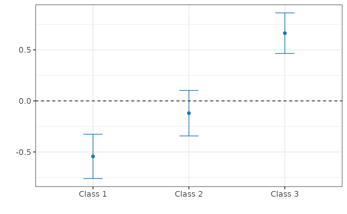
#> ── Point estimates and 95\% confidence intervals ──
#> 
#> Class 1: -0.543  [-0.760, -0.326]
#> Class 2: -0.120  [-0.343,  0.103]
#> Class 3:  0.663  [ 0.465,  0.862]
plot(fit)