Causal Inference for Qualitative Outcomes under Regression Discontinuity

Fit local polynomial regression models for qualitative outcomes to estimate the probabilities of shift at the cutoff.

causalQual_rd(Y, running_variable, cutoff)

Arguments

Y: Qualitative outcome. Must be labeled as $\{1, 2, \dots\}$.
running_variable: Running variable determining treatment assignment.
cutoff: Cutoff or threshold. Units with running_variable < cutoff are considered controls, while units with running_variable >= cutoff are considered treated.

Value

An object of class causalQual.

Details

Under a regression discontinuity design, identification requires that the probability mass functions for class $m$ of potential outcomes are continuous in the running variable (continuity). If this assumption holds, we can recover the probability shift at the cutoff for class $m$:

$$\delta_{m, C} := P(Y_i (1) = m | Running_i = cutoff) - P(Y_i(0) = m | Running_i = cutoff).$$

causalQual_rd applies, for each class $m$, standard local polynomial estimators to the binary variable $1(Y_i = m)$. Specifically, the ruotine implements the robust bias-corrected inference procedure of Calonico et al. (2014) (see the rdrobust function).

References

Di Francesco, R., and Mellace, G. (2025). Causal Inference for Qualitative Outcomes. arXiv preprint arXiv:2502.11691. doi:10.48550/arXiv.2502.11691 .

Author

Riccardo Di Francesco

Examples

## Generate synthetic data.
set.seed(1986)

data <- generate_qualitative_data_rd(100, outcome_type = "ordered")

Y <- data$Y
running_variable <- data$running_variable
cutoff <- data$cutoff

## Estimate probabilities of shift at the cutoff.
fit <- causalQual_rd(Y, running_variable, cutoff)

summary(fit)
#> 
#> ── CAUSAL INFERENCE FOR QUALITATIVE OUTCOMES ───────────────────────────────────
#> 
#> ── Research design ──
#> 
#> Identification:          Regression Discontinuity 
#> Estimand:                Probability Shifts at the Cutoff 
#> Outcome type:            
#> Classes:                 1 2 3 
#> N. units:                100 
#> Fraction treated units:  0.51 
#> 
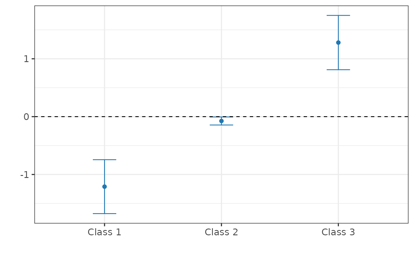
#> ── Point estimates and 95\% confidence intervals ──
#> 
#> Class 1: -1.210  [-1.676, -0.744]
#> Class 2: -0.075  [-0.145, -0.006]
#> Class 3:  1.281  [ 0.811,  1.750]
plot(fit)