Introduction to causalQual
Riccardo Di Francesco
causalQual-short-tutorial.RmdIntroduction
This tutorial provides an overview of the core functions in the
causalQual package, which facilitates causal inference with
qualitative outcomes under four widely used research designs:
-
causalQual_soo()for selection-on-observables designs -
causalQual_iv()for instrumental variables designs -
causalQual_rd()for regression discontinuity designs -
causalQual_did()for difference-in-differences designs
Each function enables the estimation of well-defined and interpretable causal estimands while preserving the identification assumptions specific to each research design.
Notation
- denotes the outcome of interest, which can take one of qualitative categories. These categories may exhibit a natural ordering but lack a cardinal scale, making arithmetic operations such as averaging or differencing ill-defined.
- denote the outcome of interest at time , with denoting the pre-treatment period and denoting the post-treatment period.
- is a binary treatment indicator.
- is a vector of pre-treatment covariates.
- is a binary instrument.
- denotes a unit’s compliance type (always-taker, never-taker, complier, defier).
- are the potential outcomes as a function of treatment status.
- are the potential outcomes as a function of treatment status and instrument assignment.
- are the potential treatments as a function of instrument assignment.
- denotes the conditional probability of observing outcome category given treatment status and covariates .
- represents the propensity score.
Selection-on-observables
Selection-on-observables research designs are used to identify causal effects when units are observed at some point in time, some receive treatment, and we have data on pre-treatment characteristics and post-treatment outcomes. This approach is based on the following assumptions:
- Assumption 1 (Unconfoundedness): .
- Assumption 2 (Common support): .
Assumption 1 states that, after conditioning on , treatment assignment is as good as random, meaning that fully accounts for selection into treatment. Assumption 2 mandates that for every value of there are both treated and untreated units, preventing situations where no valid counterfactual exists.
Together, these assumptions enable the identification of the Probability of Shift (PS), defined as
PS characterizes how treatment affects the probability distribution over outcome category . For instance, indicates that the treatment increases the likelihood of observing outcome category , while implies a decrease in the probability mass assigned to caused by the treatment. By construction, , reflecting the intuitive trade-off that an increase in the probability of some outcome categories must be offset by a decrease in others.
For illustration, we generate a synthetic data set using the
generate_qualitative_data_soo function. Users can modify
the parameters to generate data sets with different sample sizes,
treatment assignment mechanisms (randomized vs. observational), and
outcome types (multinomial or ordered).
- Setting
outcome_type = "multinomial"generates a multinomial categorical outcome (e.g., brand choices, employment status). - Setting
outcome_type = "ordered"generates an ordered categorical outcome (e.g., survey responses ranging from “strongly disagree” to “strongly agree”).
## Generate synthetic data.
n <- 2000
data <- generate_qualitative_data_soo(n, assignment = "observational", outcome_type = "ordered")

Y <- data$Y
D <- data$D
X <- data$X
Once the data set is generated, we use causalQual_soo to
estimate the PS for each outcome category. This function performs
estimation by applying the double machine learning procedures of
Chernozukov et al. (2018) to the binary variable
.
Specifically, for each class
,
we define the doubly robust scores as
causalQual_soo constructs plug-in estimates
of
by replacing the unknown
,
,
and
with consistent estimates
,
,
and
obtained via
-fold
cross fitting, with
selected by the users via the K argument.1 The estimator for PS
is then
and its variance is estimated as
causalQual_soo uses these estimates to construct confidence
intervals using conventional normal approximations.
To estimate the conditional class probabilities
,
causalQual_soo adopts multinomial machine learning
strategies when the outcome is multinomial and the honest ordered
correlation forest estimator when the outcome is ordered (Di Francesco,
2025), according to the user’s choice of outcome_type. The
function trains separate models for treated and control units. The
propensity score
is estimated via an honest regression forest (Athey et al., 2019).
causalQual_soo returns an object of class
causalQual. Generic
summary,print, and plot methods
have been extended to accommodate this class.
## Estimation.
fit <- causalQual_soo(Y, D, X, outcome_type = "ordered")
## Summary.
summary(fit)
>
> ── CAUSAL INFERENCE FOR QUALITATIVE OUTCOMES ───────────────────────────────────
>
> ── Research design ──
>
> Identification: Selection-on-Observables
> Estimand: Probability Shifts
> Outcome type: ordered
> Classes: 1 2 3
> N. units: 2000
> Fraction treated units: 0.52
> ── Point estimates and 95\% confidence intervals ──
> Class 1: -0.585 [-0.624, -0.547]
> Class 2: -0.018 [-0.064, 0.027]
> Class 3: 0.604 [ 0.565, 0.642]
## Plot.
plot(fit)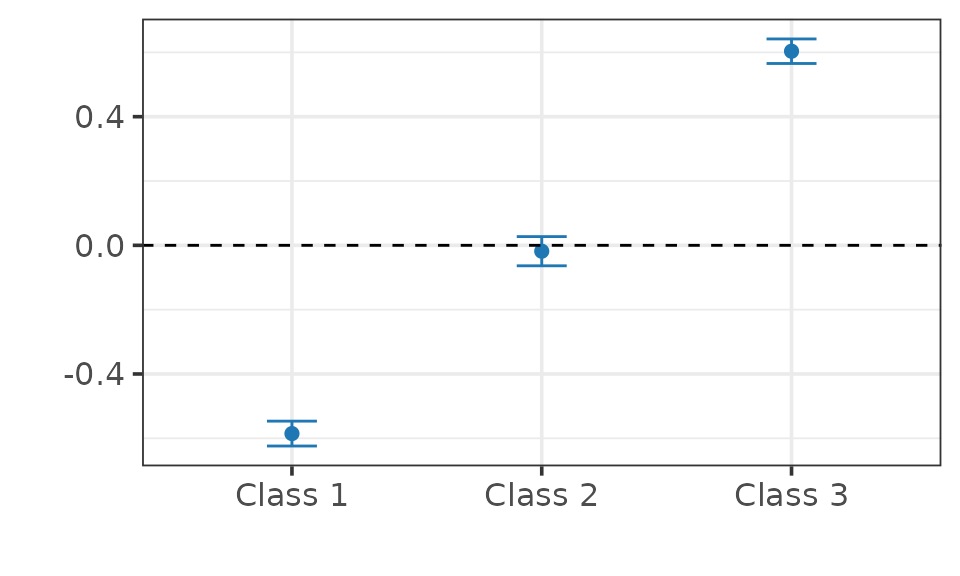
Instrumental variables
In some applications, the observed covariates may not fully account for selection into treatment, making a selection-on-observables design unsuitable. Instrumental variables (IV) designs provide a popular identification strategy to address this issue. The key idea behind IV is to exploit a variable – an instrument – that is as good as randomly assigned, influences treatment assignment, but has no direct effect on the outcome except through treatment. This exogenous source of variation enables the identification of causal effects by isolating changes in treatment status that are not driven by unobserved factors.
Formally, IV designs rely on the following assumptions.
- Assumption 3 (Exogeneity): .
- Assumption 4 (Exclusion restriction): .
- Assumption 5 (Monotonicity): .
- Assumption 6 (Relevance): .
Assumption 3 mandates that the instrument is as good as randomly assigned. Assumption 4 requires that the instrument affects the outcome only through its influence on treatment, ruling out any direct effect. Assumption 5 imposes that the instrument can only increase the likelihood of treatment, ruling out defiers.2 Finally, Assumption 6 states that the instrument has a nonzero effect on the treatment, thereby generating exogenous variation in the latter.
Together, these assumptions enable the identification of the Local Probability of Shift (LPS), defined as
LPS provides the same characterization as the PS while focusing on the complier subpopulation.
For illustration, we generate a synthetic data set using the
generate_qualitative_data_iv function. Users can modify the
parameters to generate data sets with different sample sizes and outcome
types (multinomial or ordered) as before, although
generate_qualitative_data_iv does not allow to modify the
treatment assignment mechanism.
## Generate synthetic data.
n <- 2000
data <- generate_qualitative_data_iv(n, outcome_type = "ordered")

Y <- data$Y
D <- data$D
Z <- data$Z
Once the data set is generated, we use causalQual_iv to
estimate the LPS for each outcome category. This function performs
estimation by applying the standard two-stage least squares method to
the binary variable
.
Specifically, we first estimate the following first-stage regression
model via OLS:
and construct the predicted values . We then use these predicted values in the second-stage regressions:
A well-established result in the IV literature is that, under Assumptions 3-5, (Imbens and Angrist, 1994; Angrist et al., 1996). Therefore, we estimate the second-stage regression models via OLS and use the resulting estimate as an estimate of . Standard errors are computed using standard procedures and used to construct conventional confidence intervals.3
As in the previous case, causalQual_iv returns an object
of class causalQual compatible with standard generic S3
methods.
## Estimation.
fit <- causalQual_iv(Y, D, Z)
## Summary.
summary(fit)
> ── CAUSAL INFERENCE FOR QUALITATIVE OUTCOMES ───────────────────────────────────
>
> ── Research design ──
>
> Identification: Instrumental Variables
> Estimand: Local Probability Shifts
> Outcome type:
> Classes: 1 2 3
> N. units: 2000
> Fraction treated units: 0.514
> ── Point estimates and 95\% confidence intervals ──
> Class 1: -0.632 [-0.730, -0.533]
> Class 2: 0.037 [-0.072, 0.146]
> Class 3: 0.594 [ 0.495, 0.694]
## Plot.
plot(fit)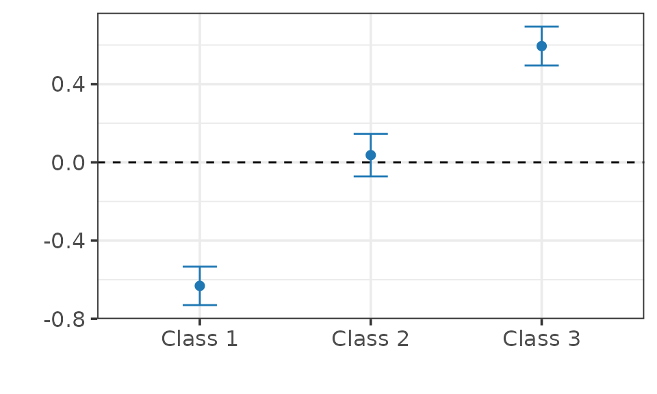
Regression discontinuity
Regression Discontinuity designs are employed to identify causal effects when treatment assignment is determined by whether a continuous variable crosses a known threshold or cutoff. The key assumption is that units just above and just below the cutoff are comparable, meaning that any discontinuity in outcomes at the threshold can be attributed to the treatment rather than to pre-existing differences.
In this section, we let be a single observed covariate (rather than a vector of covariates) and we call it “running variable.” By construction, fully determines treatment assignment. Specifically, units receive treatment if and only if their running variable exceeds a predetermined threshold . Thus, .
By construction, Assumption 1 above is satisfied since conditioning on fully determines . For our identification purporses, we introduce an additional assumption.
- Assumption 7 (Continuity): is continuous in for .
Assumption 7 requires that the conditional probability mass functions of potential outcomes evolve smoothly with . This ensures that class probabilities remain comparable in a neighborhood of .
Assumptions 1 and 7 enable the identification of the Probability of Shift at the Cutoff (PSC) for class , defined as
PSC provides the same characterization as the PS while focusing on the subpopulation of units whose running variable values are “close” to the cutoff .
For illustration, we generate a synthetic data set using the
generate_qualitative_data_rd function. Users can modify the
parameters to generate data sets with different sample sizes and outcome
types (multinomial or ordered) as before, although
generate_qualitative_data_rd does not allow to modify the
treatment assignment mechanism.
## Generate synthetic data.
n <- 2000
data <- generate_qualitative_data_rd(n, outcome_type = "ordered")

Y <- data$Y
running_variable <- data$running_variable
cutoff <- data$cutoff
Once the data set is generated, we use causalQual_rd to
estimate the PSC for each outcome category. This function performs
estimation using standard local polynomial estimators applied to to the
binary variable
.
Specifically, causalQual_rd implements the robust
bias-corrected inference procedure of Calonico et al. (2014).4
Again, causalQual_rd returns an object of class
causalQual compatible with standard generic S3
methods..
## Estimation.
fit <- causalQual_rd(Y, running_variable, cutoff)
## Summary.
summary(fit)
> ── CAUSAL INFERENCE FOR QUALITATIVE OUTCOMES ───────────────────────────────────
>
> ── Research design ──
>
> Identification: Regression Discontinuity
> Estimand: Probability Shifts at the Cutoff
> Outcome type:
> Classes: 1 2 3
> N. units: 2000
> Fraction treated units: 0.5065
> ── Point estimates and 95\% confidence intervals ──
> Class 1: -0.646 [-0.791, -0.502]
> Class 2: 0.086 [-0.067, 0.239]
> Class 3: 0.549 [ 0.392, 0.706]
## Plot.
plot(fit)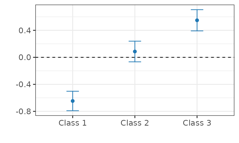
Difference-in-differences
Difference-in-Differences designs are employed to identify causal effects when units are observed over time and treatment is introduced only from a certain point onward for some units. The key assumption is that, in the absence of treatment, the change in outcomes for treated units would have mirrored the change observed in the control group.
For our identification purporses, we introduce the following assumption.
- Assumption 8 (Parallel trends): .
Assumption 8 requires that the probability time shift of for class follows a similar evolution over time in both the treated and control groups.
Assumptions 8 enables the identification of the Probability of Shift on the Treated (PST) for class , defined as
PSt provides the same characterization as the PS while focusing on the subpopulation of treated units.
For illustration, we generate a synthetic data set using the
generate_qualitative_data_did function. As before, users
can modify the parameters to generate data sets with different sample
sizes, treatment assignment mechanisms (randomized vs. observational),
and outcome types (multinomial or ordered).
n <- 2000
data <- generate_qualitative_data_did(n, assignment = "observational", outcome_type = "ordered")

Y <- data$Y
D <- data$D
unit_id <- data$unit_id
time <- data$time
Once the data set is generated, we use causalQual_did to
estimate the PST for each outcome category. This function performs
estimation by applying the canonical two-group/two-period DiD method to
the binary variable
.
Specifically, consider the following linear regression model:
A well-established result in the DiD literature is that, under Assumption 8, . Therefore, we estimate the above model via OLS and use the resulting estimate as an estimate of . Standard errors are clustered at the unit level and used to construct conventional confidence intervals.
As before, causalQual_did returns an object of class
causalQual compatible with standard generic S3
methods..
## Estimation.
fit <- causalQual_did(Y, D, unit_id, time)
## Summary.
summary(fit)
> ── CAUSAL INFERENCE FOR QUALITATIVE OUTCOMES ───────────────────────────────────
>
> ── Research design ──
>
> Identification: Difference-in-Differences
> Estimand: Probability Shifts on the Treated
> Outcome type:
> Classes: 1 2 3
> N. units: 2000
> Fraction treated units: 0.4975
> ── Point estimates and 95\% confidence intervals ──
> Class 1: -0.571 [-0.620, -0.521]
> Class 2: -0.063 [-0.114, -0.011]
> Class 3: 0.633 [ 0.595, 0.671]
## Plot.
plot(fit)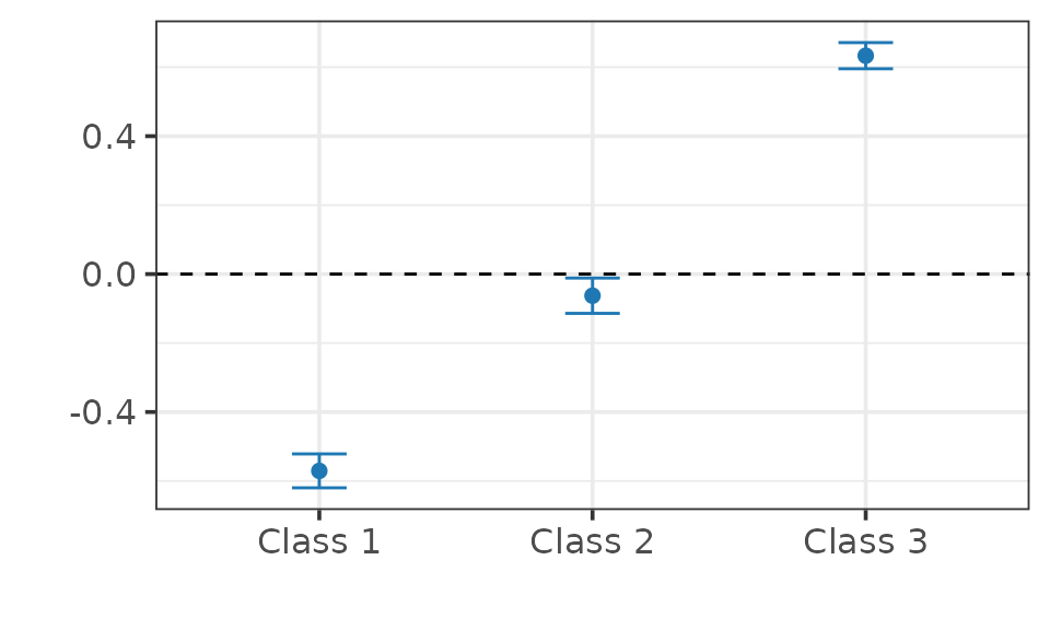
A potential issue in estimation arises if, after splitting the sample into folds and each fold into treated and control groups, at least one class of is unobserved within a given fold for a specific treatment group. To mitigate this issue,
causalQual_soorepeatedly splits the data until all outcome categories are present in each fold and treatment group.↩︎This assumption is made without loss of generality; one could alternatively assume that the instrument can only decrease the probability of treatment.↩︎
causalQual_ivimplements this two-stage least squares procedure by calling theivregfunction from the R packageAER.↩︎causalQual_rdimplements these methodologies by calling therdrobustfunction from the R packagerdrobust(Calonico et al., 2015).↩︎