Tutorial

Riccardo Di Francesco

Introduction

This tutorial provides an overview of the core functions in the ocf package, which facilitates predictive modeling of ordered non-numeric outcomes:

• ocf() for estimation and inference about conditional choice probabilities
• marginal_effects() for estimation and inference about covariates’ marginal effects

Ordered choice models

We postulate the existence of a latent and continuous outcome variable $Y_i^*$, assumed to obey the following regression model:

$$Y_i^* = g \left( X_i \right) + \epsilon_i$$ where $X_i$ consists of a set of raw covariates, $g \left( \cdot \right)$ is a potentially non-linear regression function, and $\epsilon_i$ is independent of $X_i$.

An observational rule links the observed outcome $Y_i$ to the latent outcome $Y_{i}^*$ using unknown threshold parameters $- \infty = \zeta_0 < \zeta_1 < \dots < \zeta_{M - 1} < \zeta_M = \infty$ that define intervals on the support of $Y_i^*$, with each interval corresponding to one of the $M$ categories or classes of $Y_i$:

$$\zeta_{m - 1} < Y_i^* \leq \zeta_{m} \implies Y_i = m, \quad m = 1, \dots, M$$

The statistical targets of interest are the conditional choice probabilities:

$$p_m \left( X_i \right) := \mathbb{P} \left( Y_i = m | X_i \right)$$

and the marginal effect of the $j$-th covariate on $p_m \left( \cdot \right)$:

$$\nabla^j p_m \left( x \right) := \begin{cases} \frac{\partial p_m \left( x \right)}{\partial x_j}, & \text{if } x_j \text{ is continuous} \\ p_m \left( \lceil x_j \rceil \right) - p_m \left( \lfloor x_j \rfloor \right), & \text{if } x_j \text{ is discrete} \end{cases}$$ where $x_j$ is the $j$-th element of the vector $x$ and $\lceil x_j \rceil$ and $\lfloor x_j \rfloor$ correspond to $x$ with its $j$-th element rounded up and down to the closest integer.

Code

For illustration purposes, we generate a synthetic data set. Details about the employed DGP can be retrieved by running help(generate_ordered_data).

## Generate synthetic data.
set.seed(1986)

n <- 2000
data <- generate_ordered_data(n)

sample <- data$sample
Y <- sample$Y
X <- sample[, -1]

table(Y)
> Y
>   1   2   3 
> 679 655 666

head(X)
>            x1 x2          x3 x4         x5 x6
> 1 -0.04625141  0  0.95196649  1  0.6678908  0
> 2  0.28000082  1  2.04083053  0  0.2508728  0
> 3  0.25317063  0  2.06547193  1 -0.8435355  1
> 4 -0.96411077  0 -0.02678352  0  0.2401109  1
> 5  0.49222664  0 -1.31251674  0  0.5411830  1
> 6 -0.69874551  0 -0.06783879  0 -0.8246243  1

Conditional probabilities

To estimate the conditional probabilities, the ocf function constructs a collection of forests, one for each category of Y (three in this case). We can then use the forests to predict out-of-sample using the predict method. predict returns a matrix with the predicted probabilities and a vector of predicted class labels (each observation is labelled to the highest-probability class).

## Training-test split.
train_idx <- sample(seq_len(length(Y)), floor(length(Y) * 0.5))

Y_tr <- Y[train_idx]
X_tr <- X[train_idx, ]

Y_test <- Y[-train_idx]
X_test <- X[-train_idx, ]

## Fit ocf on training sample. Use default settings.
forests <- ocf(Y_tr, X_tr)

## Summary of data and tuning parameters.
summary(forests)
> Call: 
> ocf(Y_tr, X_tr) 
> 
> Data info: 
> Full sample size:   1000 
> N. covariates:      6 
> Classes:            1 2 3 
> 
> Relative variable importance: 
>    x1    x2    x3    x4    x5    x6 
> 0.324 0.109 0.281 0.056 0.194 0.036 
> 
> Tuning parameters: 
> N. trees:           2000 
> mtry:               3 
> min.node.size       5 
> Subsampling scheme: No replacement 
> Honesty:            FALSE 
> Honest fraction:    0

## Out-of-sample predictions.
predictions <- predict(forests, X_test)

head(predictions$probabilities)
>         P(Y=1)    P(Y=2)     P(Y=3)
> [1,] 0.1580823 0.4010153 0.44090239
> [2,] 0.5871019 0.2276974 0.18520066
> [3,] 0.5416146 0.3308320 0.12755331
> [4,] 0.3369383 0.5792799 0.08378179
> [5,] 0.1066391 0.3533131 0.54004772
> [6,] 0.4305637 0.5112663 0.05817006

table(Y_test, predictions$classification)
>       
> Y_test   1   2   3
>      1 195 118  57
>      2  98 118 102
>      3  39  80 193

To produce consistent and asymptotically normal predictions, we need to set the honesty argument to TRUE. This makes the ocf function using different parts of the training sample to construct the forests and compute the predictions.

## Honest forests.
honest_forests <- ocf(Y_tr, X_tr, honesty = TRUE)

honest_predictions <- predict(honest_forests, X_test)
head(honest_predictions$probabilities)
>         P(Y=1)    P(Y=2)    P(Y=3)
> [1,] 0.1115188 0.2933057 0.5951755
> [2,] 0.5538789 0.2478605 0.1982606
> [3,] 0.3834688 0.4418804 0.1746508
> [4,] 0.5219917 0.3478453 0.1301631
> [5,] 0.1647595 0.3233609 0.5118797
> [6,] 0.3312435 0.4883800 0.1803764

To estimate standard errors for the predicted probabilities, we need to set the inference argument to TRUE. However, this works only if honesty is TRUE, as the formula for the variance is valid only for honest predictions. Notice that the estimation of the standard errors can considerably slow down the routine. However, we can increase the number of threads used to construct the forests by using the n.threads argument.

## Compute standard errors. Do not run.
# honest_forests <- ocf(Y_tr, X_tr, honesty = TRUE, inference = TRUE, n.threads = 0) # Use all CPUs.
# head(honest_forests$predictions$standard.errors)

Covariates’ marginal effects

To estimate the covariates’ marginal effects, we post-process the conditional probability predictions. This is performed by the marginal_effects function that can estimate mean marginal effects, marginal effects at the mean, and marginal effects at the median, according to the eval argument.

## Marginal effects at the mean.
me_atmean <- marginal_effects(forests, eval = "atmean") # Try also 'eval = "atmean"' and 'eval = "mean"'.
print(me_atmean) # Try also 'latex = TRUE'.
> ocf marginal effects results 
> 
> Data info: 
> Number of classes:    3 
> Sample size:          1000 
> 
> Tuning parameters: 
> Evaluation:           atmean 
> Bandwidth:            0.1 
> Number of trees:      2000 
> Honest forests:       FALSE 
> Honesty fraction:     0 
> 
> Marginal Effects: 
>    P'(Y=1) P'(Y=2) P'(Y=3)
> x1   0.222   0.081  -0.303
> x2  -2.575   1.869   0.706
> x3  -0.205   0.408  -0.203
> x4  -0.482   0.747  -0.264
> x5   0.054   0.261  -0.314
> x6   0.000   0.000   0.000

plot(me_atmean)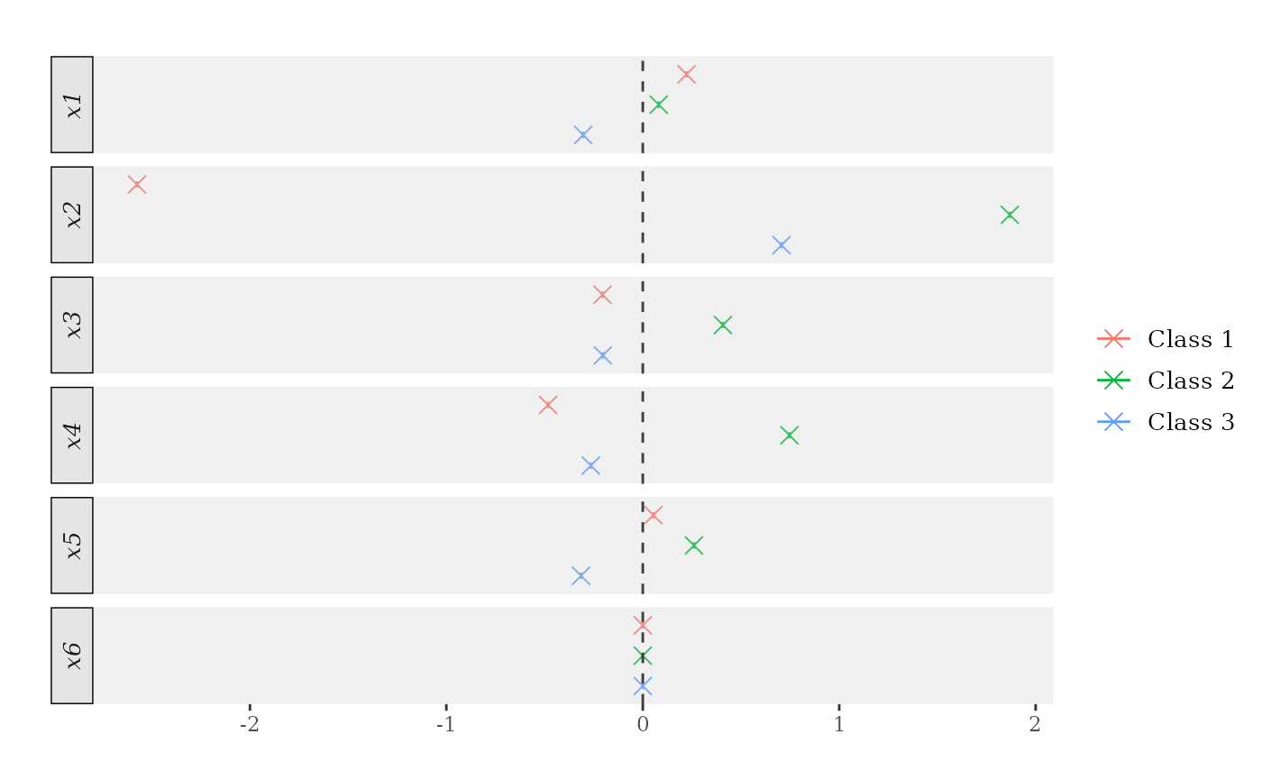

Sometimes, we are only interested in the marginal effects of a subset of the available covariates. To spare some time, we can use the these_covariates argument to estimate marginal effects of only those covariates. This argument also allows the user to declare whether the covariates are to be treated as "continuous" of "discrete" (marginal effect estimation is handled differently according to the covariate’s nature). these_covariates must be a named list, with entries’ names specifying the target covariates and entries specifying the covariates’ types. If not used, covariates’ types are inferred by the routine using basic heuristics (as in the example above).

## Marginal effects at the mean.
target_covariates <- list("x1" = "continuous", "x2" = "discrete", "x4" = "discrete")
me_atmean <- marginal_effects(forests, eval = "atmean", these_covariates = target_covariates) 

plot(me_atmean)

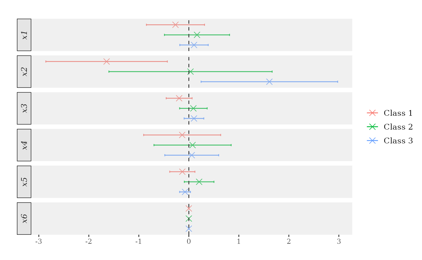
As before, we can set the inference argument to TRUE to estimate the standard errors. Again, this requires the use of honest forests and can considerably slow down the routine.

## Compute standard errors.
honest_me_atmean <- marginal_effects(honest_forests, eval = "atmean", inference = TRUE)
print(honest_me_atmean) # Try also 'latex = TRUE'.
> ocf marginal effects results 
> 
> Data info: 
> Number of classes:    3 
> Sample size:          1000 
> 
> Tuning parameters: 
> Evaluation:           atmean 
> Bandwidth:            0.1 
> Number of trees:      2000 
> Honest forests:       TRUE 
> Honesty fraction:     0.5 
> 
> Marginal Effects: 
>    P'(Y=1) P'(Y=2) P'(Y=3)
> x1  -0.267   0.163   0.104
> x2  -1.645   0.034   1.611
> x3  -0.194   0.091   0.103
> x4  -0.133   0.075   0.058
> x5  -0.130   0.206  -0.076
> x6   0.000   0.000   0.000

plot(honest_me_atmean)